The Challenge
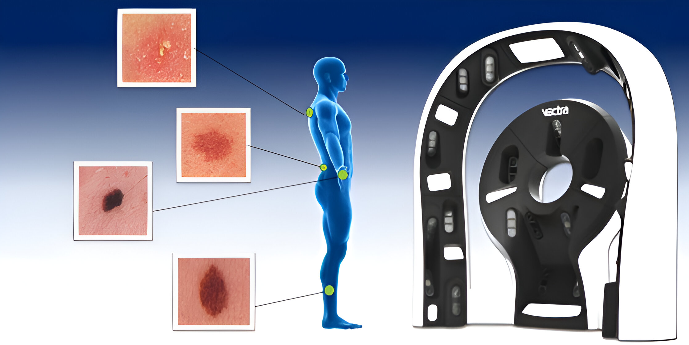
Skin cancer can be deadly if not caught early, but many populations lack specialized dermatologic care. Over the past several years, dermoscopy-based AI algorithms have been shown to benefit clinicians in diagnosing melanoma, basal cell, and squamous cell carcinoma. However, determining which individuals should see a clinician in the first place has great potential impact. Triaging applications have a significant potential to benefit underserved populations and improve early skin cancer detection, the key factor in long-term patient outcomes.
This competition challenged our team to develop AI algorithms that differentiate histologically-confirmed malignant skin lesions from benign lesions on a patient. Our work will help to improve early diagnosis and disease prognosis by extending the benefits of automated skin cancer detection to a broader population and settings.
The Plan
Our project was comprised of 3 separate models: a gradient-boosted decision tree, a visual transformer, and a final fusion model. The fusion model would take the outputs of the gradient-boosted decision tree and visual transformer as inputs and give us a final prediction. In this way, we were able to incorporate both tabluar and visual data into our model in order to obtain an optimal prediction.
The Data
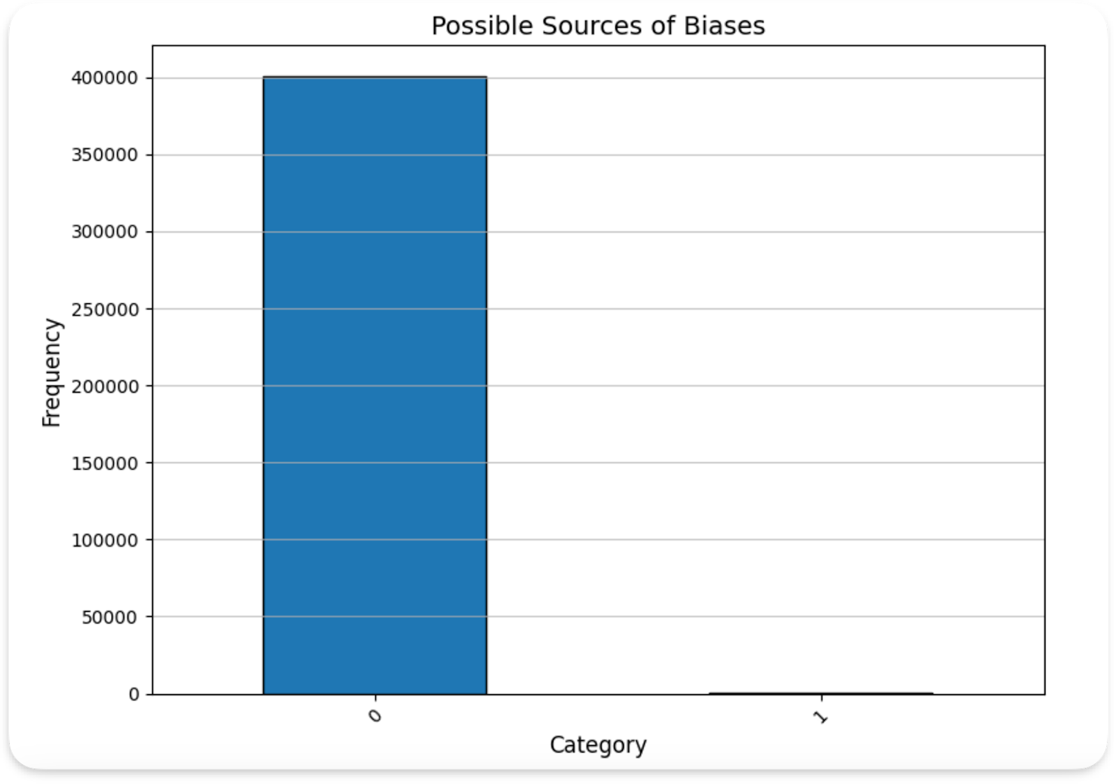
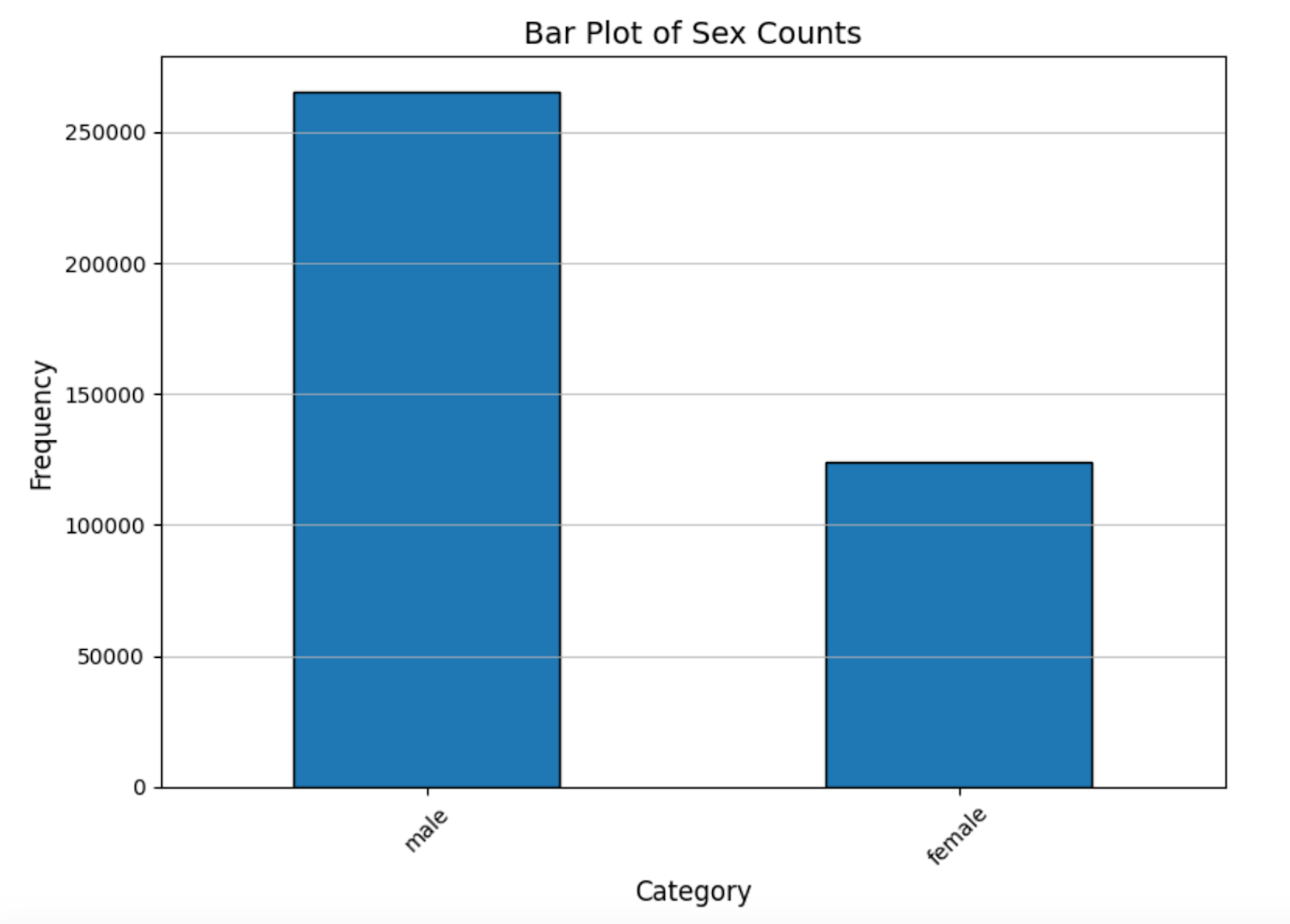
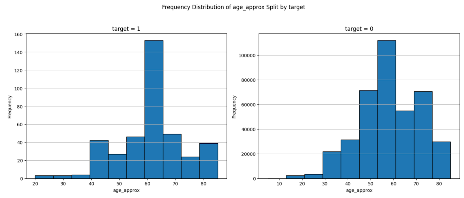
The main problem with the dataset was its skewness: nearly 99 percent of the cases are non-malignant, with 400666 non-malignant and 393 malignant data points. If we trained on this whole dataset we would start overfitting to non-malignant. We also looked for other sources of biases that may exist in the data arising from sex, age, body region. We found there to be bias in the data with respect to sex, with nearly twice the number of males to females in the training set. Additionally, the distribution of the lower body part shows a slight skew in distribution, with the posterior torso leading the count. Finally, we found the training dataset to be skewed towards older patients, with >50% of participants being over the age of 50. This makes sense as the risk of skin cancer grows with the amount of exposure to direct sunlight, something that grows with age, still, we conclude that our model will have fundamental limitations and shouldn’t be used to predict skin cancer in young individuals.
Overall, after this initial dive into the statistics of the data we decide on sampling from the data to create a more balanced dataset with respect to the target variable. Additionally, we must caution users of the model with the training biases so that it isn’t misguidedly used.
The Models
Let’s look at the 3 models designed in the project:
Gradient-Boosted Decision Tree (XGBoost)
The tabular data was imported as a dataframe. Rows containing null values were dropped to ensure data integrity. Non-informative string columns were discarded, while the remaining categorical string columns were one-hot encoded into binary vectors across unique labels. Among several location columns indicating body sites, the column with a median number of unique labels was selected to balance the trade-off between informational gain and the number of one-hot encoded columns added to the dataframe.
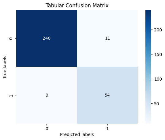
An XGBoost parallel tree boosting classifier was then trained on the cleaned dataset to classify cases as malignant or benign. Initially, the data exhibited an extreme skew toward negative labels, leading to high accuracy in predicting negative cases but very low accuracy for positive cases. To address this imbalance, a substantial portion of the negative label rows was removed to adjust the class distribution. The classifier was retrained on this adjusted dataset, resulting in high accuracy for both positive and negative cases. The final confusion matrix is given below.
The final model achieved an accuracy of 93.63% with an AUC of 0.9067.
Visual Transformer (ViT)
The model is structured around a Visual Transformer (ViT) that takes in 224x224 images as tensors and produces a softmax layer for classification. The model “splits an image into fixed-size patches, linearly embeds each of them, adds position embeddings, and feeds the resulting sequence of vectors to a standard Transformer encoder. In order to perform classification, [the model] uses the standard approach of adding an extra learnable “classification token” to the sequence” (Dosovitskiy). We chose a transformer as a model due to its proven track record at image classification and because of its fast learning rate.
In order to train the model on our data, some preprocessing is required. The original images are first read as byte strings, which are converted into images and then resized. The model then takes these as input and produces a softmax layer of size n, where n is the number of classes. The Visual Transformer is pre-trained with model weights from ‘vit-base-patch 16-224-in21k’. This ensures the model has a basic understanding of images, which helps the model identify key features in our images. This also means that less training is required.
To test the model, we created a test subset of the data prior to training. The confusion matrix shows the accuracy for 1000 predictions from that set. It shows strong accuracy when differentiating negative cases. However, it struggles with positive cases. This is likely due to class imbalance. The training data is heavily skewed towards negative cases, thus providing much more information for negative cases. Even when class imbalance was accounted for, there is still a slight bias towards negative cases.
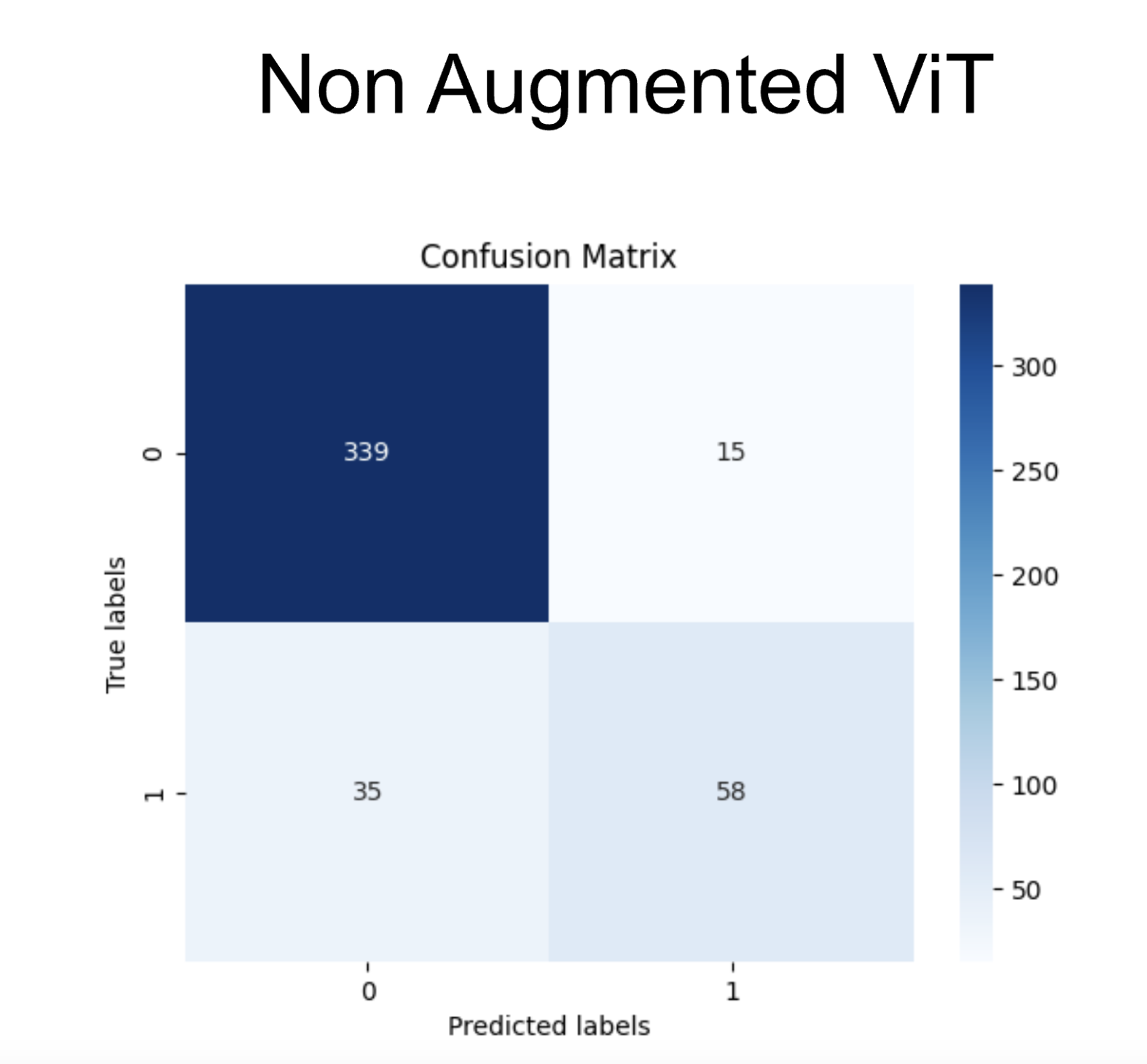
Image Augmentation
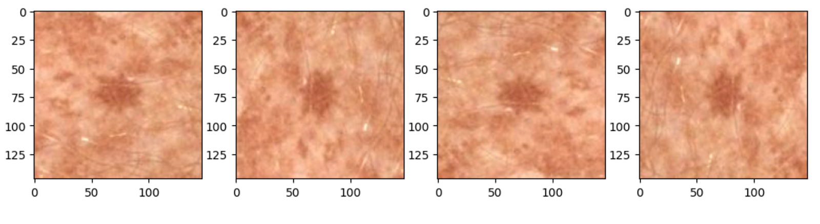
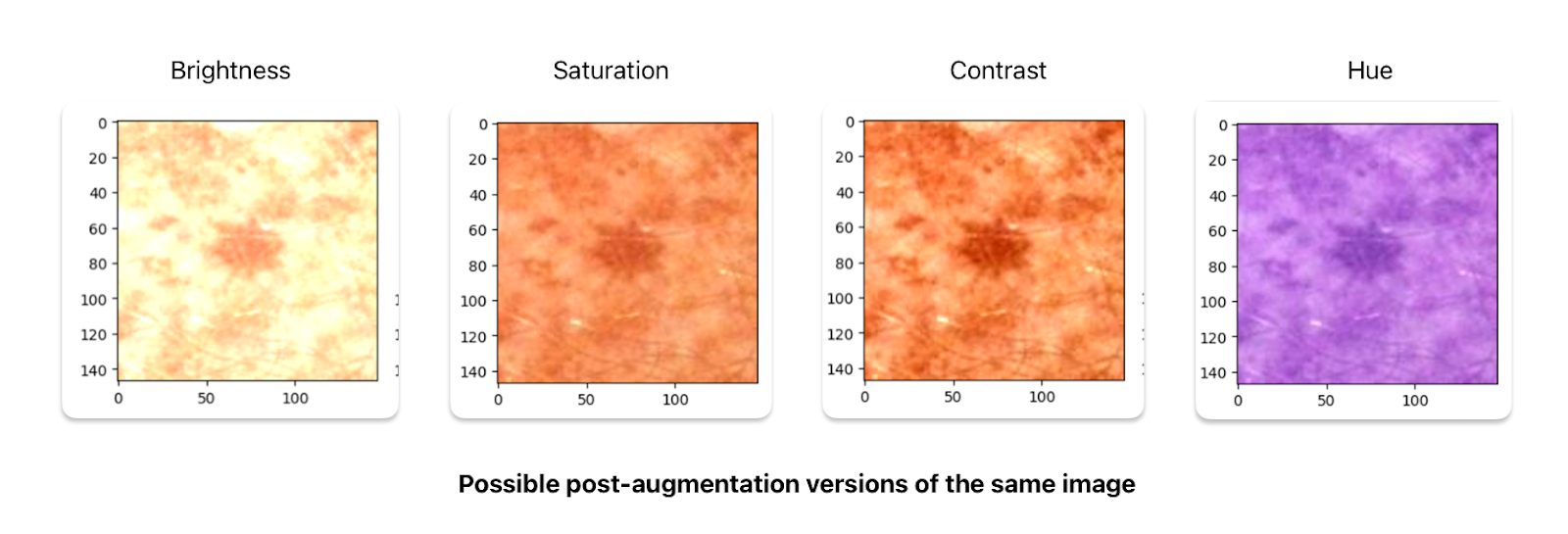
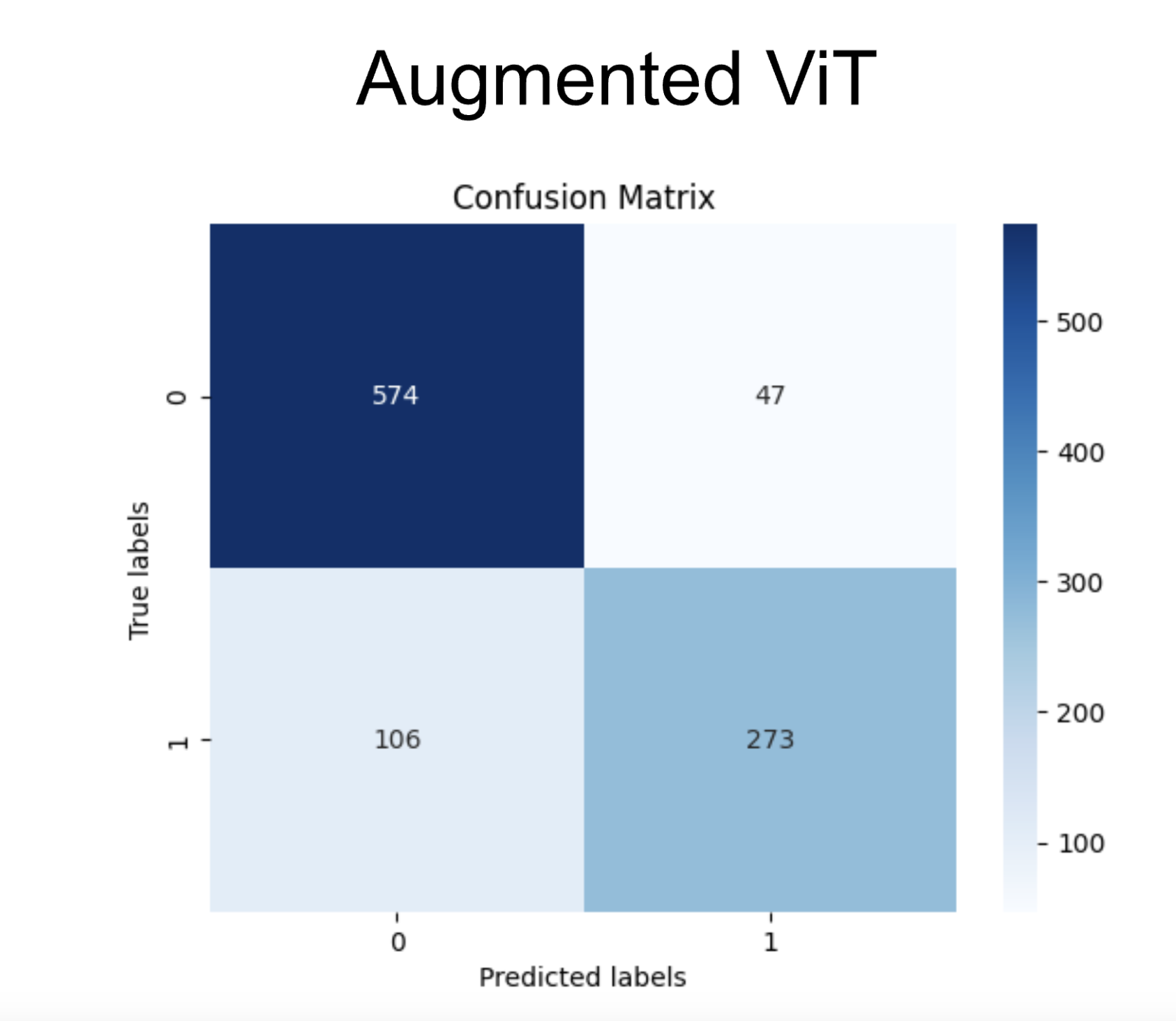
In order to improve the model, we tried a myriad of data augmentation techniques. This included rotating and recoloring the image to increase our training size. We specifically constructed an augmented training set, which was approximately 3x the size of the original training set. We did so by adding two new modified sets, which we will refer to as the rotation set and the color-jittered set. Together they formed a training set size of 8460. To create these modified sets we create copies of the original set and sample a transformation. The rotation consisted of 4 possible rotation transformations: {0,90,180,270}. The color jittered set was inspired by a few blog posts we found (check the GitHub for examples and sources) and consisted of 4 possible augmentations to an image: saturation, hue, contrast, and brightness. Here are some figures showing what a specific image may look like after the transformations:
After training the ViT model on the augmented dataset we found a slight improvement in the model. After performing K Fold cross validation, we found the best k to be 5 (out of 5). After performing evaluation, we found the accuracy of the ViT pre-augmentation to be .85, with an ROC curve shown above and an AUC of .791. The accuracy on the augmented ViT was found to be .88, up 3 percent from the original non-augmented accuracy.
Fusion Model
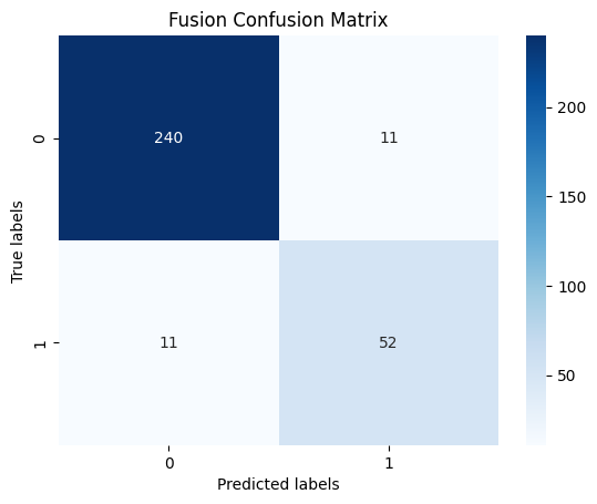
To achieve fusion, we combined the final output layers of our Vision Transformer (ViT) model (without the augmentations) and added them to our tabular data and put that into an XGBoost model. These outputs of the ViT represented probabilities of detecting skin cancer. Since the ViT model updated its parameters based on the validation set, using k-fold cross-validation as an evaluation metric could introduce data leakage. To mitigate this, we reused the same training and validation splits from the previous model, choosing fold k=4, where the same fold served as the validation set in the ViT. In this setup, the validation set was treated as a proxy for the test set.
As shown in the figures below, this model obtained high levels of success, reaching an AUROC of 0.8907 and 92.99% accuracy on the validation set, scores that outperformed our other models. The only downside to this model was that there was only an 82.5% accuracy on positive results, which may be dude to the class bias. However, these results were still extremely impressive and were tied with the tabular model as the best of the models that we used.
The Results
In our experimentation, we found that the tabular model outperformed the visual model. We found this somewhat counterintuitive, as the image data seemed to be the most direct representation of the classification. However, the tabular model performed noticeably better than the visual mode, with an accuracy of 93.63 and 84.5 respectively. This may be due to a lack of visual identifiers in the images as well as obstructions in the images. Thus, despite the lack of visual information, there may have been features of the tabular data that do a better job of identifying benign and malignant targets. The fusion model outperformed the tabular on average but suffered from the lack of CV. We could not apply CV to since it could only be trained on the same fold as the vision model to prevent data leakage. The increase in average performance between the tabular and fusion shows that the visual method learns information not present in the tabular data.
Additionally, the class imbalance of the data had an immense effect on the performance of the models. Prior to class imbalance, the data distribution was 99.902134 (0) and 0.097866 (1). To combat this, we adjusted the distribution of the target classes by using specified sampling fractions to under-sample the majority class (0) while including all samples of the minority class (1). After rebalancing, data had a distribution of 80 (0) and 20 (1). This drastically improved our models’ performance and allowed them to better differentiate the minority class (1). Our original method for the distribution adjustment upsampled the minority class by repeating samples, which introduced data leakage. Although we aren’t able to work with as much data because of this, the move to only downsample the majority class has resolved this data leakage issue.
Finally, we implemented K-Fold Cross Validation (KFCV) into our models. K-Fold Cross Validation is a technique that divides the dataset into multiple folds, using each fold as a test set once while the remaining folds are used for training, to ensure robust evaluation of model performance. For the ViTs, we split the data into 5 folds, with 5 models corresponding to a different test fold. We compared the results for each model and selected the model with the best performance.
After running KFCV on the ViT model and the tabular models, we saw the following results. The best models were chosen for each method.
| K-Fold | 5 | 4 | 3 | 2 | 1 |
| Image Model Accuracy | 0.850 | 0.979 | 0.894 | 0.947 | 0.967 |
| Tabular Model accuracy | 0.9013 | 0.9172 | 0.9268 | 0.9363 | 0.9299 |
| Tabular Model AUC | 0.835 | 0.847 | 0.871 | 0.907 | 0.891 |
Although there are many things we can improve, we were very happy with our final model’s performance.
GitHub
Full Code and explanation can be found at our GitHub.